A review of third quarter reports from hedge funds finds that, at least as of September 30, many event-driven managers continue to seek much of their equity-like exposure through positions in distressed or discounted but still performing credits. The extent to which this is a deliberate choice based on strategic considerations is not in all cases clear.
Strategies of seeking equity-like exposure through the credit markets has had much to recommend them over the last couple of years, and dedicated investors in distressed situations are likely to continue to seek such exposure. But returns on these investments tend to be slow to develop and “lumpy.” It could be that, in many cases, the continued predominance of credits in event-driven portfolios simply reflects the fact that investments made a year or two ago have yet to achieve their return targets. Retention of a bias toward credits could also be a matter of liquidity: even at the best of times, most such instruments are fairly illiquid, and if the prospect that they will achieve their return targets are fading, demand for them is likely to be even less. Managers who might otherwise allocate away from them may be deterred by the necessity of having to accept steep discounts in order to liquidate them.
Distress and discounted performing credits are always with us, but their supply varies, as does their inherent attractiveness. The opportunity to acquire the paper of sound borrowers at steep discounts occurs only during times of crisis – the credit spreads on such paper have narrowed since the Credit Crunch, and where liquidity allowed, most such positions acquired at that time have probably been realized. There is always new supply of distressed debt, as previously healthy firms encounter difficulty, but the quality of a borrower that enters into distress at a time of relative economic calm is rather different from that of a borrower whose distress results from global macroeconomic dislocation. Widespread distress offers opportunity to hedge funds that are not distressed debt specialists. As the new supply of distressed debt arises increasingly from firms that fall into distress for idiosyncratic, firm-specific rather than macroeconomic reasons, fewer managers other than distressed debt specialists will be attracted to it.
All this suggests that many hedge funds’ allocation toward credits will decrease over time, almost certainly in favor of an increased allocation to equities. The credit positions they have built over the last few years will either attain their return targets and be liquidated or gradually be abandoned. Specialists will continue to plough the debt furrow, but the majority of event-driven managers are likely to find more opportunity in trades employing equities rather than equity-surrogates. Other factors support this trend – most notably the high levels of liquidity on corporate balance sheets. This encourages corporations to create opportunities for merger arbitrage, a tendency that is already clearly in place, and in an environment where arbitrageurs face less competition from private market buyers than they have in the recent past. Where they are not used to finance acquisitions, cash hoards invite corporate activism, in which many event-driven managers delight. The U.S. environment for activism will improve next year, thanks to changes to proxy rules. In the next year or so, strategies involving equities can be expected to bulk larger in event-driven portfolios than they have recently.
Tuesday, November 9, 2010
Monday, October 11, 2010
Life Settlements Returning to Life?
The Wall Street Journal reported on October 9 that Leon Black’s Apollo Global Management is raising a $525 million fund to invest in life settlements, and the Financial Times notes that similar funds are being marketed in Europe. According to an SEC staff report, this rather obscure investment category has seen investor interest halve since its 2008 peak, when $15 billion in face value was transacted, but these high-profile fund raisings suggest that it may be reviving.
Investors in life settlements buy an actuarially diversified pool of life insurance policies from their owners. Payment for them is above surrender value but at a negotiated discount to face value, which is currently around 87%. Purchasers pay the policy premia (5 - 10% of face value per year) until the demise of the insured, at which point they claim the policies’ face value from the insurers that issued them.
Apart from the returns it can offer, the principal attraction of this type of investment is that it has little correlation to any other: it provides an income stream that is unrelated to security market trends, and since it is self-liquidating, exit involves uncertainty only as to timing and not as to the price that will be achieved. For example, a single policy purchased at 13% of face value with a 5% annual premium will return a compound annual rate of 17.5% if the insured expires after seven years. Obviously, the rate of return is strongly influenced by actual mortality outcomes: in this example, the return would be 23.4% if death occurs in six years and 13.3% if it occurs in eight. Thus the principal risk involved in life settlements relates to the soundness of the actuarial assumptions underlying the construction of the basket of policies purchased. If properly constructed, the same assumptions imply that later premia can be covered by earlier mortalities, making the position self-financing after a few years.
There are various reasons why life settlements have never attracted enormous investor interest and have recently fallen further out of favor. Not least are controversy and complex litigation surrounding policy acquisition practices, many of which have been questionable in the past. The industry has established codes of conduct, most states have legislated on these matters, and one of the recommendations of the SEC staff paper mentioned above was that life settlements should be brought within the definition of ‘security,’ which would allow federal regulation by the SEC. Thus uncertainty regarding investors’ title to policies should be in the process of resolution. However, this will not address issues regarding the return structure of these investments.
Consider the highly simplified caricature of a life settlement fund in the chart below. It consists of 500 policies with a face value of $1 million each, on the lives of average American males who simultaneously turned age 75 at the start of year one. Mortality assumptions are drawn from the Social Security Administration’s Period Life Table for 2006. The policies are purchased at an 87% discount to face value and each has a $50,000 annual premium. To keep matters simple, premium payments, receipt of death benefits accumulated over the course of the year and income distributions all occur on the last day of each year.

The compound annual return on this hypothetical investment is a very respectable 12.4% over thirty years. However, it is rather slow in coming: cumulative return is negative, dipping as low as -6.8% at the end of year two, and first turns positive at the end of year five. Premium payments due exceed death benefits received by $4.4 million in the first two years, so the first distribution is received at the end of year three. The investment does not return the initial $65 million investment until year eleven. In short, life settlements exhibit a fairly extreme J-curve, which is bound to limit investor interest in them to those with long investment horizons and the patience to wait for the first glimmer of a return. While this makes them sound ideal for many institutional purposes, it is an unusual (if exemplary) investment committee that can tolerate negative returns for five years and still have achieved only a 9.2% compound return after ten.
Of course, this example is contrived: real funds have much greater actuarial diversity. If the basket of policies includes some on older people or viatical settlements – that is, policies on people with a life expectancy of less than two years (the 75-year olds in the example have an average life expectancy of 10.5 years at time zero) – the investment’s unproductive period can be reduced. However, the J-curve cannot be completely eliminated. Regardless of the construction of the policy basket, life settlements will remain suitable only to patient investors.
So the audience for the funds being launched is rather limited, and it is unlikely that many such vehicles will be offered successfully. This is unfortunate, because many of the policies in the new crop of funds will be purchased from banks that need the liquidity. While there has been some discussion of securitization of life settlements (another reason for the SEC’s interest), most industry commentators seem to think that this is an unlikely development. Again, the return profile explains why. This also is unfortunate: despite the whiff of sulfur around an investment activity that appears to gamble on peoples’ deaths, and which has sometimes been characterized by dubious practices in the past, a more economic alternative to surrendering their policies is a very real benefit to some of the insured. While the life settlement market is unlikely ever to become big, it is not a bad thing that there is at least some life in it yet.
Wednesday, September 29, 2010
Correlation Trading
Members of the option community have for some years touted implied volatility as the “new asset class,” so it was probably inevitable that their creative energies would turn to implied correlation as the “new, new asset class.” Volatility is relatively easy to trade, using options straddles, for example, and the CBOE’s 2003 launch of the “new” VIX Index and related derivatives, which are essentially just synthetic straddles, simply offered convenience rather than a revolutionary new opportunity to traders. Structuring option positions that provide directional exposure to correlation is more difficult, and such trades were uncommon among any but the most sophisticated option arbitrageurs until the designers at the CBOE launched the S&P 500 Implied Correlation Index last year.
The Index is a synthetic dispersion trade. In a structure that is bullish on correlation, long positions in call options on a basket of index components are hedged with short positions in calls on the index. A bearish view on correlation would reverse the long and short positions. It is essential that the basket of long calls be optimized to replicate the trading behavior of the index as closely as possible – the CBOE Index employs fifty positions, rebalanced monthly – which explains why relatively few traders exploited this structure in the past. The way the structure works is that the index position hedges away the β of the individual components, so that what remains is their specific risk. When this decreases relative to their β, correlation increases; when it increases relative to their β, correlation declines.
Predictably, correlation counter-correlates with the underlying S&P 500 Index, but not nearly as much as volatility does: the coefficient of correlation was -0.4075 for the January 2011 Correlation Index (11/25/08 - 9/27/10; ticker JCJ) compared to -0.7280 for the VIX Index. Also as would be expected, correlation was considerably less volatile than the VIX during the same period (annualized standard deviations of 47.9% and 110.9%, respectively), although it is somewhat surprising that correlation had nearly twice the 26.5% volatility exhibited by the underlying S&P 500 Index.
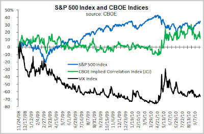
As with the VIX Index, it is important to remember that the Correlation Index is an option-implied statistic, and that its value as a predictor of actual outcomes is limited. Both tend to imply outcomes that are higher than they actually turn out to be, although they may on occasion undershoot the actual outcome, as they both have done recently. An article by Theo Casey in Futures and Options Intelligence (requires registration) argues that the current high levels of correlation can be ascribed to ETF trading, and there may be some merit in this. However, he also raises the possibility that this heralds a fundamental change in the structure of the equity markets. However, the high levels of activity in ETFs are themselves a result of current market conditions, and likely to change. Over its 23 month life, JCJ has traded as low as 19.92 and as high as 81.09. It does not seem likely that it is the bellwether of a consistently highly correlated market.
Saturday, September 18, 2010
Prime Office Real Estate
Institutional interest in prime office buildings has been strong since the end of last year. This is not surprising: cap rates (annual lease rates ÷ capital costs) are high, while the yield on competing investments in quality corporate bonds is hardly compelling. There is a widespread perception that prime locations can be picked up at distressed prices, offering the prospect of capital gain in addition to a solid income stream. Vacancy rates in most markets, while elevated, are not extreme, and there is little supply coming on stream from new construction in most of them, suggesting that lease rates will remain firm provided that vacancies do not rise. There are reasonable grounds for confidence that they will not, if only because they have failed to do so during the worst of the recession: lessees are either warehousing space for future needs or using space less intensively than they had in recent years. Finally, the inflation-protective aspect of real estate is attracting institutions that require current income (such as those with distribution requirements), since they are otherwise challenged to find such protection from income-producing instruments other than TIPS.
Thus the investment case in favor of office real estate is fairly strong, and prime structures, which have always attracted the bulk of institutional real estate interest, are the principle beneficiaries of it. General Partners of private real estate vehicles have been quick to launch new funds to accommodate this interest. However, investors in these funds are likely to find that it is difficult for their General Partners to find investments in which to deploy their capital. Property owners are naturally resistant to selling at what they also perceive as depressed prices. The flood of distressed selling that many investors anticipated has not materialized, as lenders have preferred to renegotiate rather than to foreclose, doubtless influenced by the same perception of the potential value of their collateral, as well as the substantial costs of foreclosure. The gradual recovery of the CMBS market will do nothing to discourage this preference, since it increases the liquidity of lenders’ positions and offers the prospect that, if they need to, lenders will be able to exit their positions on better terms than they could achieve through foreclosure and re-sale. As is frequently the case with depressed real estate markets, there is a constellation of interests that prevents the market from clearing rapidly. Thus opportunities to acquire prime office properties cheaply are less abundant than many institutions had expected.
 The inevitable result will be that returns on the current vintage of prime office funds will be less than their most optimistic investors had hoped. Will they be less than their required rates of return? From the trough in Q4 1993 to the peak in Q2 2008 shown in the chart above, annual total returns from office properties were a quite satisfactory 8.9%, while for the whole period shown, including two drawdowns of 23% and 36%, the total return was a still-respectable 5.9%. The recent slump was more severe than the 1990 - 1993 decline, and recovery has been more rapid. Fundamental conditions – cap and vacancy rates, foreseeable newbuilding – support a return forecast that is at least as attractive as the 1993 - 2008 trough-to-peak experience. The major imponderable is the behavior of investors themselves. If institutional money continues to flood into the prime office sector, and owners continue to resist distressed sales, much of the price recovery will redound to the benefit of the existing owners and their creditors rather than the current vintage of new funds.
The speed with which returns have begun to recover suggests that this is precisely what is happening. If their required return is above, say, 6.5%, uncommitted investors would probably be wise to broaden their real estate search beyond prime U.S. office space to other building types, geographies or investment strategies. For example, the state of the market in the prime segment suggests that conditions for “value added” investment in office structures – those that require refurbishment – are close to ideal. Of course, if the “value added” office segment attracts significant institutional inflows, this will further dampen returns on prime office buildings, since the effect of “value added” investment is to increase the supply of prime office space through repositioning the buildings purchased.
Thus the investment case in favor of office real estate is fairly strong, and prime structures, which have always attracted the bulk of institutional real estate interest, are the principle beneficiaries of it. General Partners of private real estate vehicles have been quick to launch new funds to accommodate this interest. However, investors in these funds are likely to find that it is difficult for their General Partners to find investments in which to deploy their capital. Property owners are naturally resistant to selling at what they also perceive as depressed prices. The flood of distressed selling that many investors anticipated has not materialized, as lenders have preferred to renegotiate rather than to foreclose, doubtless influenced by the same perception of the potential value of their collateral, as well as the substantial costs of foreclosure. The gradual recovery of the CMBS market will do nothing to discourage this preference, since it increases the liquidity of lenders’ positions and offers the prospect that, if they need to, lenders will be able to exit their positions on better terms than they could achieve through foreclosure and re-sale. As is frequently the case with depressed real estate markets, there is a constellation of interests that prevents the market from clearing rapidly. Thus opportunities to acquire prime office properties cheaply are less abundant than many institutions had expected.

The speed with which returns have begun to recover suggests that this is precisely what is happening. If their required return is above, say, 6.5%, uncommitted investors would probably be wise to broaden their real estate search beyond prime U.S. office space to other building types, geographies or investment strategies. For example, the state of the market in the prime segment suggests that conditions for “value added” investment in office structures – those that require refurbishment – are close to ideal. Of course, if the “value added” office segment attracts significant institutional inflows, this will further dampen returns on prime office buildings, since the effect of “value added” investment is to increase the supply of prime office space through repositioning the buildings purchased.
Saturday, September 11, 2010
CalPERS’ Proposed Investment Classification
As mentioned in my book, CalPERS has been studying the idea of reclassifying its investments for the purpose of adding clarity to its asset allocation efforts. Pensions & Investments Online reports that CalPERS suggests the reclassification shown below, although this may not be its final form: the proposal is contained in a memo that will be considered at a November meeting of its Investment Committee, and differs from an earlier proposal that was floated in March.
 The reclassification is clearly a move away from an asset class-based schema toward a more functional classification of investments. Although the old classification included one category – inflation-protective – that is clearly functional in nature, the new classification includes four functional categories, with only “real assets” as an asset class-based category.
The inadequacies of an asset class-based schema are abundantly clear to any Investment Committee that has struggled with one, and CalPERS has made a laudable attempt to circumvent them. It would be unfair to nit-pick over the proposed reclassification, since it may still be subject to modification, the details of how its categories will be defined remain unclear and how allocation based upon them will be implemented has not been discussed. However, it is not just an aesthetic objection that the proposed reclassification retains an asset class-based category.
The point of a functional classification is to underline the portfolio role of the instruments that comprise the investable universe. The function-based categories that CalPERS has defined pretty much cover the essential tasks that a portfolio must perform on behalf of the institution:
• to preserve capital against inflation and deflation or credit crisis;
• to provide current income to meet distribution requirements and to enhance tactical flexibility; and
• to increase the endowment to allow the institution to expand its activities if its trustees so choose.
Many, if not most, investments exhibit characteristics that help fulfill more than one of these functions – dividends, for instance, provide income from the “growth” allocation that is surely welcome. But this can be accommodated within the schema by distinguishing between investments’ primary and secondary portfolio roles. So where does the asset class-based category of “real assets” fit in? Investments in this category will presumably be selected in order to perform one or more of the essential portfolio functions – if not, why allocate to them at all? So CalPERS’ unwillingness to follow the logic of its proposed classification system and restrict itself to four functional categories seems inconsistent.
The advantage of functional classification is that it puts first things first: optimization among asset classes is not the first priority of an Investment Committee. Before it reaches any decisions regarding the disposition of its assets, a Committee should ponder what it wants to accomplish with the resources at hand. For example, if it is an inescapable duty to make a 7% distribution of assets in each of the next three years, questions of the disposition of its portfolio resources must follow from that requirement. If it is an immature defined benefit program, the Committee is instead likely to focus on the pursuit of growth. The appropriate asset allocation follows from such decisions, so classifying investments by their portfolio function aids the Investment Committee in performing its primary task.
It is in this context that CalPERS’ retention of a “real assets” category seems odd. Maintaining positions in real assets is not a function that an institution needs to accomplish: they, like any other investments, are means to an end. Timberland and infrastructure are primarily income-producing investments, but with a measure of inflation protection. Real estate as a broad category encompasses prime office buildings, with similar characteristics, but also development projects that more closely resemble growth equity. The logic of CalPERS’ classification schema suggests that investment categories that fall under “real assets” should be redistributed.
There is at least one category of investments – one so-called asset class – that poses significant challenges to CalPERS’ functional schema: “absolute return.” Presumably it provides some protection against inflation (if it cannot produce a real return, why invest in it at all?). A real return is clearly a minimum requirement for investments that fit into the “growth” category, but investments that can only meet this minimum standard represent rather poor candidates for fulfilling the function of increasing the endowment. Although its returns may be “absolute” in most market conditions, its tail risks tend to be closely related to those of the assets on which its strategies are employed, so its adequacy as a hedge is debatable. Few such investments provide current income. CalPERS’ proposal has generated some controversy, and I suspect that not the least reason for this is that it cannot find a natural classification for “absolute return.” This begs the question of whether this is in fact a flaw, or carries the unexpected implication that “absolute return” does not fulfill any essential portfolio functions very well.
Sunday, September 5, 2010
Reports of the Death of Mean Reversion are Exaggerated
Many investment strategies employ techniques that identify potentially attractive trades on the assumption that prices revert to a central trend, generally referred to as a ‘mean,’ although it may not actually have that mathematical pedigree. The claim for these techniques is that prices can be expected to pull back from the extremes to which supply or demand may push them, and that isolating a sufficiently stable central tendency allows traders to identify and exploit such reversions. For at least a year now, this assumption has been under strain in various markets.
Before proceeding further, however, there is a red herring to dispose of. In an August 2 Financial Times editorial, Richard Clarida and Mohamed El-Erian of Pimco muddy the waters by arguing from the extreme dispersion of current economic opinion – deflation vs. hyperinflation, recovery vs. recession – to the conclusion that investors will flee investment techniques that rely on some historical measure of value to which prices revert. Their reasoning is unsound. From a wide disparity of economic expectations it follows that there is a wide disparity of opinion on where value is to be found – but it does not follow that value itself is widely dispersed. Value is a matter of economic outcomes, not economic perceptions. Some forecasts will turn out to be correct, leading their adherents to value and attractive returns, while others will turn out to be wrong, suggesting value where in fact there is none (the bond market, perhaps?). Confusion over the economic outlook may cause investors to despair over their ability to identify sources of value, but it does not follow that there is no value to be found.
The issue regarding mean reversion does not relate to valuation but to technical analysis and algorithmic trading, particularly over the short time horizons employed by high frequency traders and statistical arbitrageurs. By definition, any procedure used to derive a central price tendency – whether it is a moving average, the arithmetic mean relative to which standard deviation is calculated, or what-have-you – must take time series data for its inputs. The longer the time series – the greater the number of observations used in the function or algorithm used to define the tendency – the less volatile the central value will be. That is, the longer the series, the less the next observation will cause the trend to shift, even if it diverges very sharply from the tendency. The effect of this “dilution” of recent observations can be compensated by various methods of weighting them more heavily than earlier ones, but it cannot be completely eliminated.
Since they are unavoidably lagging indicators, in periods of high volatility these central tendencies may not be of much value to traders. This is especially true when markets are volatile over several time horizons – day to day, week to week and month to month – and when their volatility is itself volatile, increasing and decreasing rapidly. In the charts below, standard deviation is calculated over ninety observations, which is about the shortest series that allows for statistical significance. It does not take much imagination to see why it would be difficult for mean reversion techniques to thrive in the U.S. equity market since April of this year. For much of the period those who rely on mean reversion were subject to frequent false signals or no meaningful signals at all.

All investment managers experience periods during which their discipline is not rewarded by their market’s characteristics. In some cases these periods can be quite protracted, inevitably causing them much soul-searching and not a little despondency. Managers without access to alternative trade identification procedures to fall back on may even be forced to close shop before conditions become more favorable to them. But conditions will eventually change, and if in the meantime the ranks of traders reliant on mean reversion trading signals have been thinned, the reward to mean reversion techniques will be that much greater.
Friday, August 27, 2010
Risk Arbitrage and Leveraged Buyouts
The current rash of high profile acquisitions has, inevitably, raised speculation about an impending merger boom. This is probably a bit premature. While some of the conditions that would encourage a boom, such as corporate cash levels, borrowing costs and the equity valuations of potential targets are favorable to deal-making, equity volatility and concern about the economic outlook are likely to instill caution in boardrooms, at least for the time being. The value of U.S. deals announced year to date still lags behind the same period of 2009, which was itself a very soft year. While transaction volume outside of the U.S. has been stronger (and risk arbitrage is a global activity), so far this year it has managed to boost global year-to-date activity only marginally over 2009 levels. In part because of the cyclicality of their trade – recent experience is hardly the first merger drought − many of these traders are now ensconced within “event-driven” hedge funds, which have other strategies such as distressed investing or convertible arbitrage that they can pursue if the merger cycle is unfavorable.
These circumstances would suggest that things are improving somewhat for risk arbitrageurs, if not dramatically. However, although it seems unlikely that merger activity could quickly return to the frenetic pace of 2005 - 7, conditions may in fact be improving more rapidly for risk arbitrageurs than the headline statistics would suggest. The reason is that the composition of current deal-flow is more favorable to them than it was during the buyout boom. Risk arbitrageurs are benefiting from the problems of the leveraged buyout funds.
An arbitrage requires at least two tradable legs – one long and one short. When an acquirer is a private entity such as an LBO fund, and thus does not trade, no arbitrage may be possible. This is not always the case – for example, if the target’s debt trades at a discount, and its debt covenants have a change-of-control provision that requires an acquirer to repurchase the debt at par, a risk arbitrage may still be possible (long the debt/short the equity). However, even if such a trade is possible, it is a rather narrow one, because the amount of the relevant debt outstanding is, in almost all cases, a fraction of the deal size. It is difficult to estimate how much of the acquisitive activity during 2005 - 7, when LBO funds dominated the merger market, actually offered trading opportunities to risk arbitrageurs. At a guess, it was only 65% of the value of deals completed.
The acquisition market has changed in the meantime. LBO funds are having difficulty obtaining the amount of leverage that they could readily access during the buyout boom. In a complete reversal of their experience then, in several recent deals they were handily outbid by non-financial purchasers. Trade buyers’ can raise debt far more easily and cheaply than LBO firms in the current environment. Although some of the most powerful LBO firms continue to be able to complete large deals, LBO funds in general are concentrating more of their attention on middle-market transactions. This is a segment that generally offers less compelling opportunities to risk arbitrageurs than large and complex deals, since arbitrage is most attractive to pursue where liquidity is ample.
The opportunities available to risk arbitrageurs are not measured solely in terms of transaction size: the premium that the acquirer ultimately pays for the target is also a crucial metric. Recent experience has also been quite favorable to them in this respect. Contested bids, such as those that feature in several current transactions, can also expand their opportunities, although at some cost in terms of increased risk. Hedge funds that are equipped to exploit these opportunities – whether risk arbitrage specialists or more diversified “event-driven” firms – may not be experiencing a golden age, but this is certainly a productive period for them.
Monday, August 23, 2010
High Frequency Trading and the "Flash Crash"
It requires only a glance at securities industry job sites to see that high frequency trading continues to grow rapidly, even though it is already thought to account for half of U.S. equity volume. The “Flash Crash” of May 6 and subsequent regulatory interest in these activities have attracted media attention to this corner of the markets. The technicalities of market microstructure and the use of computer algorithms, machine learning, etc. in an attempt to exploit it would seem unlikely to capture the public imagination. But the topic has a certain sci-fi glamour, which is enhanced by the perceptions that markets have escaped human understanding, that events such as the one pictured below could easily recur, and that participants in this activity are up to no good. Mystery, the threat of catastrophe and a suspicion of scandal – how could a journalist (or for that matter, a Congressman) resist?
 There has been high frequency trading since the first stock exchanges opened in the seventeenth century – computerization has only accelerated its pace. As outlined in a recent IOSCO study, modern transaction speeds do raise concerns about pre-trade risk and compliance controls, but few if any of these are insurmountable. More trenchant criticisms note that high frequency trading, in the context of fragmented markets with multiple venues, each offering a somewhat different microstructure, opens the door to price manipulation and to meltdowns such as the “Flash Crash.” Further, the competition for liquidity among these venues has led to the practice of selling access to flash orders, which many commentators regard as tantamount to permission to front-run other market participants.
Dubious as the practice may be, offering firms access to flash orders is simply the latest in a long line of privileges that exchanges have offered to attract liquidity providers to their platforms. They argue that investors benefit from these, in terms of faster execution and price improvement: for example, the CBOE claims that flash orders saved its customers $3.6 million in a single month. However, if the practice is banned, as the SEC proposes, it is inevitable that exchanges will respond by devising some new trading privilege to attract liquidity providers. This is not just a cynical comment. Providing a venue for liquidity is exchanges’ business, but they are not in a position to provide it themselves, since that would transform them into broker-dealers. So they have no choice, in a competitive environment, but to find ways to attract third party liquidity to their transaction mechanisms. When exchanges argue that they perform a public service by offering privileges that enhance their liquidity, high frequency traders can hardly be blamed for making use of them.
Multiple, competing exchanges with different transaction mechanisms almost certainly do increase the opportunities for market failure, as has been apparent since the mechanics of the Crash of 1987 began to be understood. Whether computerized direct access to these execution venues exacerbates this problem is debatable. It is likely that modern market infrastructure would have prevented or at least greatly ameliorated the 1987 episode. On the other hand, while the causes of the “Flash Crash” remain obscure, it is certain (if only because of their share of transaction volume) that high frequency traders played an important role in it. While the information available to regulators may not, in the end, be sufficient firmly to establish the cause of the “Flash Crash,” this indicates a serious gap in their capabilities that must be filled – the sooner the better.
As the IOSCO paper notes, regulatory authorities are somewhat hampered with regard to the enforcement of rules against market manipulation by some of the ways that high frequency traders may obtain direct electronic access to markets. This is a situation that must be corrected. Since there is reason to suspect that tape-painting and possibly even more highly irregular activity by high frequency traders contributed significantly to the “Flash Crash,” addressing this issue must also be a high regulatory priority. Much of this can be accomplished by enforcing existing rules, provided that regulators are able to obtain the information needed in order to do so. Fortunately, this is essentially the same information they would require to determine the causes of such episodes.
Friday, August 20, 2010
Inflation and Infrastructure
Infrastructure would seem to offer investors a fairly safe refuge from inflation, and on the whole it does. Operators of infrastructure have at least some scope to raise user fees, and can expect to recoup the depreciated cost of maintenance and improvements upon exit from their position. However, some forms of infrastructure may offer more certain inflation protection than others. In particular, the ability of public infrastructure to insulate against inflation cannot in all cases be counted upon.
First, a digression on inflation, three measures of which are shown below. The best indicator for the aggregate economy is the GDP deflator. It is not more widely used because it is released with a lag – note that the figures after 2007 are still not final – and because inflation in the total economy is too broad a measure for many purposes. The CPI, although widely used, is an imperfect measure, neglecting interest costs, which account for more of consumers’ budgets than many of the items that are included, and since it calculates on a fixed basket of goods, it ignores the price elasticity of consumer demand. The third indicator is rather obscure, but it is probably the best available gauge of the cost of maintaining infrastructure. It tracks the costs of labor, equipment and materials used in heavy construction − pipelines, roads, bridges, earthworks, pumping plants, transmission lines, etc. Although it covers only the seventeen Western states within the Bureau of Reclamation’s remit, it is unlikely that the picture it creates would differ greatly if it included all fifty. The point of showing these indicators is to draw attention to the fact that different portions of the economy can experience different rates of inflation.
 The contracts under which public infrastructure is operated are fixed at the time of purchase or lease, and usually include limits on permissible increases in user fees. These will typically be linked to the CPI, the rate of inflation that is most familiar to most users. Given the political sensitivities involved, operators are often restricted to less than the increase in that Index. As the chart indicates, this can put operators of public infrastructure in a squeeze: since 2003, the Bureau of Reclamation series has risen at twice the rate of the CPI. Operators of infrastructure whose user fees can at best increase no more rapidly than CPI are experiencing deteriorating margins, which the decline in their costs in 2009 did not relieve. In principle these should be recoverable on exit from the position, but given the time horizon of infrastructure investments, that could be a long wait. In the meantime their investors experience less than perfect inflation protection on their cash flow distributions.
In contrast, operators of private infrastructure do not risk such pressures. Although the commercial relationships between providers of private infrastructure and their customers vary, pricing is in almost all cases a matter of regular negotiation. Most of their customer contracts are annual, on a take-or-pay basis. Where contracts are of longer duration, operators are generally in a position to assure themselves that any anticipated cost increases are reflected in the charges they negotiate. Providers of private infrastructure have an obvious negotiating advantage over their customers, most of whom cannot easily turn to other providers, and who therefore also have a strong interest in the maintenance of the facility. In any case, inflation is likely to affect their customers’ revenues positively, reducing their resistance to increases in usage charges provided that they are not egregious. With respect to inflation risks, operators of private infrastructure can be relied upon to take care of themselves (and their investors) to an extent that may not be possible for operators of public infrastructure.
First, a digression on inflation, three measures of which are shown below. The best indicator for the aggregate economy is the GDP deflator. It is not more widely used because it is released with a lag – note that the figures after 2007 are still not final – and because inflation in the total economy is too broad a measure for many purposes. The CPI, although widely used, is an imperfect measure, neglecting interest costs, which account for more of consumers’ budgets than many of the items that are included, and since it calculates on a fixed basket of goods, it ignores the price elasticity of consumer demand. The third indicator is rather obscure, but it is probably the best available gauge of the cost of maintaining infrastructure. It tracks the costs of labor, equipment and materials used in heavy construction − pipelines, roads, bridges, earthworks, pumping plants, transmission lines, etc. Although it covers only the seventeen Western states within the Bureau of Reclamation’s remit, it is unlikely that the picture it creates would differ greatly if it included all fifty. The point of showing these indicators is to draw attention to the fact that different portions of the economy can experience different rates of inflation.

In contrast, operators of private infrastructure do not risk such pressures. Although the commercial relationships between providers of private infrastructure and their customers vary, pricing is in almost all cases a matter of regular negotiation. Most of their customer contracts are annual, on a take-or-pay basis. Where contracts are of longer duration, operators are generally in a position to assure themselves that any anticipated cost increases are reflected in the charges they negotiate. Providers of private infrastructure have an obvious negotiating advantage over their customers, most of whom cannot easily turn to other providers, and who therefore also have a strong interest in the maintenance of the facility. In any case, inflation is likely to affect their customers’ revenues positively, reducing their resistance to increases in usage charges provided that they are not egregious. With respect to inflation risks, operators of private infrastructure can be relied upon to take care of themselves (and their investors) to an extent that may not be possible for operators of public infrastructure.
Saturday, August 14, 2010
Alternative Investments and Deflation
My previous post discussed an asset category that is widely regarded as a hedge against inflation, and subsequent efforts will return to investments that help investors preserve purchasing power. However, recent economic news has revived speculation, which has been recurrent for several years, about the possibility of deflation. Some comments on what alternative investments can do to protect investors in a deflationary environment seem to be in order.
It should come as no surprise that the answer is, “Not much.” Few investments benefit from deflation. Sovereign debt is usually regarded as a safe haven (although not a hedge) against it, but it is unclear that the debt of a nation such as the U.S., which relies so heavily on foreign purchasers to finance it, will offer such protection. Japan's experience over the last decade is not indicative: Japan is able to fund its borrowing from domestic savings. If deflation discourages foreign interest in funding what would remain of U.S. consumption, the Treasury yield curve could become quite steep despite the Fed’s best efforts. In this connection, it is not clear what deflation would do to the value of the dollar, relative to major currencies, to traditional hard currencies such as the Swiss Franc, or to gold.
A deflationary environment would, however, provide rich pickings for short-bias hedge funds and investors in distressed situations. It should also provide opportunity to macro hedge funds. This may sound odd, since the last several years’ revival in the fortunes of macro strategies has to a large extent been tied to commodity price developments. But fundamentally, macro investment exploits economic dislocation and volatility, of which there would be plenty in a deflationary scenario. High frequency trading and arbitrages (other than risk arbitrage, which would probably see its opportunities evaporate) could still be productive if volatility does not become too extreme and if sufficient leverage to make these activities remunerative is still available. Trend-following CTAs should also be able to take advantage of deflation, particularly because it is likely to be accompanied by backwardated markets, while those whose trade discovery is driven by mean-reversion would tend to have a difficult time. Most other hedge fund categories would also struggle.
Direct lenders could expect to see demand increase and competition wither, but default experience would deteriorate, and those whose loans are collateralized could find that their security is less valuable than they had thought. Deflation could plausibly launch a period of considerable prosperity for the life settlement business, with increased supply reducing acquisition costs, thus mitigating some of the J-curve effect that has plagued this investment technique recently.
Real assets could be expected to suffer under deflation − infrastructure, particularly private infrastructure − probably less so than others. Although it is firmly ensconced in the commodity sector, the agricultural economy has a cycle at least partially of its own. It is conceivable that farmland and agricultural commodities could escape the worst effects of deflation, but they cannot be relied upon to do so. The experience of the Great Depression seems to argue against optimism on this score, but U.S. agriculture had already entered depression in 1920 as a result of the post-war retreat of commodity prices: agriculture was probably more of a contributing cause than a consequence of the economy-wide deflation after 1929. The ability of timber investors to forego harvesting and income, while tonnage on the stump continues to grow, would offer a possible safe haven during a deflationary episode, provided that it was not too protracted. Unfortunately, once under way, deflation is stubbornly persistent. If deflation results in a decline in the value of the dollar, this might be expected to bolster other commodity prices, but demand destruction would probably be a greater influence on their price development.
Private equity and real estate would not thrive under deflation. Even if by some chance a private equity position does well despite the environment, neither the IPO market nor trade buyers are likely to offer an attractive exit opportunity. Mezzanine finance would probably be difficult to come by, so even a successful investment may come under stress. In a deflationary environment, lease rates would be under pressure, few buyers for real estate would be available, and refinancing, again, might be difficult to locate. In both cases, funds may also find that committed capital is not available to meet capital calls. The secondary markets for private equity and real estate vehicles are likely to see a considerable increase in supply, offering attractive discounts to funds with liquidity to deploy, but these will only provide a cushion against losses rather than an opportunity if the deflationary episode is lengthy.
By and large, alternative investments tolerate moderate inflation better than they accommodate deflation − which is equally true of conventional investments. However, some of them at least offer the hope that they can offer positive performance during a deflationary episode, which is more than conventional assets other than sovereign debt can offer. More to the point, a portfolio of alternative investments that is positioned to weather a period of deflation need not penalize the investor’s performance too dramatically if, in fact, deflation does not materialize. The same is not true of a conventional portfolio designed to protect against deflation.
Tuesday, August 10, 2010
Investment in Farmland
Investor interest in farmland has increased steadily, motivated by the perception that it offers an attractive yield, solid prospects of capital gain and inflation protection. Recent experience supports this view. Over the period shown in the first chart below, U.S. “dirt values” have increased by a compound 3.7% a year. The series is too short for statistical significance, but for what it’s worth, its standard deviation was 6.6%, which is comparable to corporate bonds. Lease rates on cropland (i.e., land that is not under lower-value pasture) have risen by a compound 2.8% annually over the shorter period shown in the second charrt. Note that these averages mask wide dispersions: average cropland values per acre differ by 28X between largely unirrigated New Mexico and potentially sub-divisible Rhode Island.
 The increase in farmland values and lease rates is generally ascribed to commodity price developments. Most investors avoid operating farms, and since most leases renew annually, investors tend to purchase properties used for growing annual crops, so that they do not actually own the biological means of production. For obvious prudential reasons, owners of property under perennials such as trees or grapevines prefer to operate the farms or employ tied agents to do so. Although some leases include a participation feature, most investors avoid such arrangements. So in fact, most investors’ returns have no direct relationship to commodity prices. However, if it has no “higher better use” (i.e., as a subdivision), the price of farmland derives from the value of what it can produce. The rental that it can command is also a function of anticipated commodity prices. So the perception that investors’ returns are largely determined by commodity price developments, with some but not excessive lag, is largely correct.
Whether commodity prices are strong or not, increasing production is the main way that a farm operator can grow its business. Farming has a high fixed cost component, so the pursuit of economies of scale is critical to commercial success, except in a few niches. American agriculture is already among the world’s most productive, so investments in increased intensity offer only diminishing returns. Thus increased scale requires increased acreage. With mortgages cheap, farm balance sheets (as shown below) healthier than they have been in a generation and fairly encouraging prospects for commodity prices, operators’ demand for farmland competes with investors’ interest in acquiring it. Farm operators are, in the nature of the case, advantaged bidders: in effect, investors compete against insiders. It seems likely from the uptick in farm leverage that they are competing with them quite actively.
 This provides additional incentive for investors to look for non-U.S. opportunities, where “dirt value” may not be so firm and where competitive bidders may not have such financial resources. However, investors generally confine themselves to regions where agriculture is fully modern. Farm operators who can still gain scale from increased expenditure on fertilizer or hybrid seed will weigh the cost of doing so against the cost of leasing or purchasing acreage. In those regions, “dirt value” and lease rates are likely to stagnate. Investment in “emerging” farming regions is best left to owner-operators, who have the skill, resources and incentive to increase the productivity of properties that they can buy comparatively cheaply there. It is best avoided by passive investors.
In the U.S. and especially elsewhere, the yields on passive agricultural investment and the potential capital appreciation that it offers remain attractive relative to corporate bonds. But the U.S. case is no longer strongly compelling. The opportunity to buy U.S. farmland at prospective total returns comparable to those available in 1987 is unlikely to recur. Consequently, the inflation-protection argument is crucial in order to make a strong case for farmland investment. That is, price expectations for agricultural commodities must be optimistic to justify investment. Otherwise, investment success in U.S. farmland must rely on opportunistic and very judicious purchase.
There are many reasons to be optimistic about the demand for agricultural commodities over the intermediate- to long-term, but given the relative inefficiency of much of the world’s farming, supply is fairly elastic. Granted, it lags demand by several years. Malthusian arguments in support of farmland investment should therefore be discounted, at least on a twenty-year view. Investors should assume that supply will be able to meet demand within the life of their investment, in the process clawing back any extraordinary gains. Since farmland is a long-tail investment, with substantial transaction costs, it should not be purchased as a short-term speculation. Although there will inevitably be supply interruptions that bolster short-term returns, such as the current Russian drought, investors in an illiquid asset are unwise to assume that they will be able to exploit them. This does not argue against investment in farmland, but given that its returns and apparent risk profile are not extraordinary, it argues very strongly in favor of strict price discipline. For most farmland investors, this means that they must rely on a highly qualified agent to handle the purchase and management of their investments.

Whether commodity prices are strong or not, increasing production is the main way that a farm operator can grow its business. Farming has a high fixed cost component, so the pursuit of economies of scale is critical to commercial success, except in a few niches. American agriculture is already among the world’s most productive, so investments in increased intensity offer only diminishing returns. Thus increased scale requires increased acreage. With mortgages cheap, farm balance sheets (as shown below) healthier than they have been in a generation and fairly encouraging prospects for commodity prices, operators’ demand for farmland competes with investors’ interest in acquiring it. Farm operators are, in the nature of the case, advantaged bidders: in effect, investors compete against insiders. It seems likely from the uptick in farm leverage that they are competing with them quite actively.

In the U.S. and especially elsewhere, the yields on passive agricultural investment and the potential capital appreciation that it offers remain attractive relative to corporate bonds. But the U.S. case is no longer strongly compelling. The opportunity to buy U.S. farmland at prospective total returns comparable to those available in 1987 is unlikely to recur. Consequently, the inflation-protection argument is crucial in order to make a strong case for farmland investment. That is, price expectations for agricultural commodities must be optimistic to justify investment. Otherwise, investment success in U.S. farmland must rely on opportunistic and very judicious purchase.
There are many reasons to be optimistic about the demand for agricultural commodities over the intermediate- to long-term, but given the relative inefficiency of much of the world’s farming, supply is fairly elastic. Granted, it lags demand by several years. Malthusian arguments in support of farmland investment should therefore be discounted, at least on a twenty-year view. Investors should assume that supply will be able to meet demand within the life of their investment, in the process clawing back any extraordinary gains. Since farmland is a long-tail investment, with substantial transaction costs, it should not be purchased as a short-term speculation. Although there will inevitably be supply interruptions that bolster short-term returns, such as the current Russian drought, investors in an illiquid asset are unwise to assume that they will be able to exploit them. This does not argue against investment in farmland, but given that its returns and apparent risk profile are not extraordinary, it argues very strongly in favor of strict price discipline. For most farmland investors, this means that they must rely on a highly qualified agent to handle the purchase and management of their investments.
Thursday, August 5, 2010
Internal Stress Tests
I argued in my July 31st posting that there are rather obvious reasons why the stress tests that regulatory authorities produce for public dissemination might fall short of the severest stringency. Authorities consequently run the risk that, if their tests that are perceived to be undemanding, they might be discredited and even counterproductive, given that publication of their results is intended as a confidence-building exercise. But of course, they also run the risk that excessively demanding tests could damage confidence. Banking authorities must tread a fine line. The same certainly should not be true of stress tests that firms devise for strictly internal consumption. Here it is self-defeating to set the parameters of stress any lower than the limits of what the firm can withstand, since the purpose of performing the tests is precisely to determine what those limits are.
The Credit Crunch revealed that stress can be extraordinarily complex. Sources of risk that are normally treated as conceptually distinct – market stress, credit stress, liquidity stress, operational stress, etc. – all seemed to manifest themselves simultaneously and in bewildering combinations, making it virtually impossible to separate primary causes from subsidiary effects. The Credit Crunch provided ample evidence, if any evidence were needed, that simple models of stress do not reflect the complex realities of systemic crises.
As in other situations, it is sound advice to “follow the money.” While the disappearance of liquidity is not usually a cause of financial crises, it is their invariable accompaniment. It is also the main proximate cause of financial stress, even illiquidity is only a subsidiary effect of whatever event originally caused the crisis. Consider the chart below, which shows the development of one the of financial system’s many sources of leverage. From the second to the third quarter of 2008, $1.1 trillion in credit was withdrawn from the system. On I.M.F. estimates, this increase exceeds all but twelve nations’ G.D.P. and equals 1.9% of the global economy. Such a massive withdrawal of liquidity cannot have failed to affect every leveraged participant in the system, even though it followed directly upon an even more massive increase from the first quarter to the second. Clearly, it would be impossible to trace all the margin calls, forced liquidations and recourses to standby credit facilities that resulted from such wholesale de-leveraging.

At the level of the individual firm, if it is even moderately complex, it is not possible to create a comprehensive test that addresses all the inter-connected sources of stress that were revealed by the Credit Crunch. Testing for stress at a level of such near-universal crisis requires a number of scenarios that increases by the square of the number of position, creditor and debtor exposures the firm carries. This figure rapidly becomes enormous. However, the firm can reduce it to more manageable size by concentrating its attention on margin calls resulting from haircuts to the values of its positions, the callable portion of its other indebtedness and to the default risk among its debtors. This is still a substantial task, but then the stress revealed during the Credit Crunch was itself very substantial. The firm that can hypothetically stress itself to this extent without reaching the limits of its solvency is in extremely sound shape.
Wednesday, August 4, 2010
Erratum
Erratum to Alternative Assets and Strategic Allocation

p. 71
Figure 3.6 was erroneously reproduced in Figure 3.7.
Figure 3.7 should appear as follows:
Saturday, July 31, 2010
European Stress Tests
The announcement of the results of Europe’s bank stress tests on July 23rd was greeted with relief and rallies in bank shares and the euro. It also sparked widespread criticism of the adequacy of the tests and cynicism regarding Europe’s cosseting of the ninety-one banks (accounting for 65% of European bank assets) that were tested. Several commentators drew unfavorable comparisons with the stress tests that were applied to U.S. banks earlier in the year. Both reactions were thoroughly predictable, but it is interesting to consider why this should be so.
Relief was largely a matter of how weak confidence in Europe has been in the wake of the Greek crisis. All the banks that failed the test – Germany’s Hypo Real Estate, Greece’s ATEBank and five Spanish savings banks – were thought to be in difficulty well before the announcement of the results. One of the Spanish cajas that failed the test even anticipated its result by issuing €450 million of convertible debt to J.D. Flowers. So the test results did nothing to add to the general gloom, and investors’ reflex reaction was to mark up prices. I am reminded of an interesting market commentary that ran on the DJ Newswire many years ago: “The market rose on lack of bad news.” Critical reactions were equally reflexive. It is to be expected that there will always be those who feel that the stress scenarios applied to the banks were not stringent enough, and who, in consequence, suspect the authorities’ motives. The justice of their objections to the E.C.B.’s methodology – among them its unwillingness to extend price haircuts to banks’ held-to-maturity positions and its debatable treatment of sovereign exposures – are to some extent neither here nor there. The simple fact that tests were performed made criticism along these lines inevitable.
All of which begs the question, how stressful should stress tests be? At some level of stress, every bank is unsound, and given empirical evidence that >20σ events can occur in financial markets, there is no a priori case for calibrating tests to any given level of stress. For all that it is recurrent and even patterned, stress is inherently improbable – otherwise it would not be stress, but business-as-usual. This is why VaR and similar measures of banks’ quotidian risks are supplemented by stress tests in the first place. Cynics argue that authorities calibrate their tests to a stress level that will guarantee that their results do no damage to confidence in the banking system. There is inevitably some truth in this: it is hardly the authorities’ intention to induce stress by testing for it. They must obviously weigh the danger of diminishing confidence through excessive stringency against the risk of discrediting the stress testing exercise. But it is not remarkable, in the current state of European banking, that a 92% pass rate, the revelation of no unexpected weaknesses in the system and an estimated aggregate capital shortfall of only €3.5 billion suggest to some commentators that the tests might appropriately have been more stringent.
The challenge to the authorities is to determine the failure rate that is consistent with the maintenance of confidence in the banking system, and what and how many unexpected test failures confidence can tolerate. The alternative is to refrain from public release of stress test results. Since public release of the test results is itself a confidence-building exercise, it is unreasonable to expect them to behave otherwise. However, it should give us pause that European authorities apparently feel that confidence is so fragile that calling attention only to well-recognized weaknesses that require only a small capital infusion to correct is all that confidence in their banking system can withstand.
Subscribe to:
Posts (Atom)